U-Net for Semantic Segmentation of Soyabean Crop Fields with SAR images.
Brazil is one of the main soyabean producers in the world, with the state of Mato Grosso being the largest producer and with the largest area of soyabeans planted. Several initiatives stand out in the mapping of soybean crop fields. An example is the GAAF/UNEMAT SojaMaps. In this post, we will try to obtain good results in mapping soyabean crop fields, using images from ESA Sentinel 1. From Google Earth Engine, we will obtain satellite images and apply the semantic segmentation technique to obtain binary images labeled in soybean and no soybean.
Semantic Segmentation
In Computer Vision Semantic Segmentation is a high-level task, which aims to understand the scene and identify to which semantic class each pixel of the image belongs. Some of those applications include self-driving vehicles, human-computer interaction, virtual reality etc. With the popularity of deep learning in recent years, many semantic segmentation problems are being tackled using deep architectures, most often Convolutional Neural Nets, which surpass other approaches by a large margin in terms of accuracy and efficiency.
SAR Images
A Synthetic Aperture Radar (SAR), or SAR, is a coherent mostly airborne or spaceborne sidelooking radar system which utilizes the flight path of the platform to simulate an extremely large antenna or aperture electronically, and that generates high-resolution remote sensing imagery. Over time, individual transmit/receive cycles (PRT’s) are completed with the data from each cycle being stored electronically. The signal processing uses magnitude and phase of the received signals over successive pulses from elements of a synthetic aperture. After a given number of cycles, the stored data is recombined (taking into account the Doppler effects inherent in the different transmitter to target geometry in each succeeding cycle) to create a high-resolution image of the terrain being over flown.
See more about SAR:
Sentinel 1
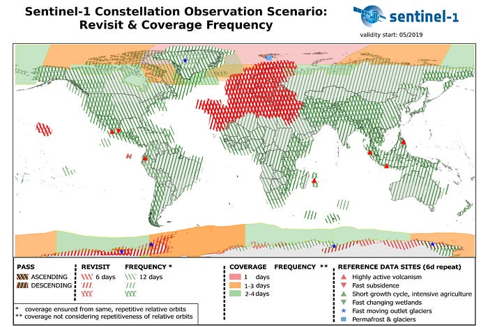
The Sentinel-1 mission comprises a constellation of two polar-orbiting satellites, operating day and night performing C-band synthetic aperture radar imaging, enabling them to acquire imagery regardless of the weather. Sentinel-1 satellites have a built-in SAR instrument that operates in the C band at a frequency of 5,405 GHz. The system has the ability to operate in dual polarization (HH / HV or VV / VH) and single polarization (HH or VV) ) and has four distinct acquisition modes: SM (Stripmap Mode), IW (Interferometric Wide Swath Mode), EW (Extra-Wide Swath Mode) and WV (Wave Mode).

Getting SAR images from Google Earth Engine
In Google Earth Engine we will select the central points for creating the polygon where the images and the respective masks will be clipped:

After selecting the collection points, we will define the Sentinel 1 VV and VH bands in 6 periods of 2019. Thus, we will have 12 spectral features to classify our images.

Finally, we clipped the image collection for each sampled area, we export the SAR data in .tif format to Google Drive along with the Sentinel 2 RGB images for the process of creating the labeled masks.
Create the labeled masks
The creation of labeled masks is a long and tiring process most of the time. In each image we must select the regions that will belong to the pre-defined classes. To facilitate this step, we will use the image segmentation platform segments.ai.
Before, we converted Sentinel 2 RGB images downloaded from gee into .png format to upload them on the segmentation platform. On the platform, we perform the segmentation and selection of regions that will be masked for each image in our dataset.

After labeled the masks, the plataform releases a .json file with the url of the binary images to download them.
Import Mask and SAR Images on Google Colab
We will use the GPU available on Google Colab to train the semantic segmentation model. First we import our images stored in Google Drive and download the labels from the aws server of the segments.ai platform. We transformed the images and labels into a numpy array to feed our model.

As we will use only a few sampling regions, we will use the technique called data augmentation, which consists of performing spatial operations such as rotation, translation, zoom etc., thus increasing the number of examples available for training the model without the need to spend more time with collection and data labeling.
Keras U-Net Model
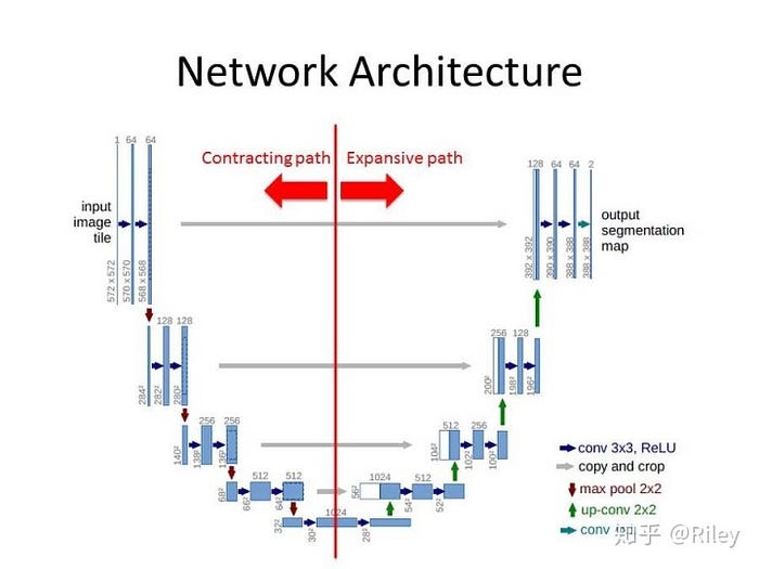
U-Net is a convolutional neural network architecture created by Ronneberger in 2015. Basically it consists of an encoder and a decoder. The encoder is responsible for extracting the main characteristics of the image, through convolution operations and for reducing its size through the pooling layers. The decoder, on the other hand, recovers the initial spatial configuration of the image by concatenating it with its respective encoder layer.

We use keras to build our U-Net according to the code below.
upconv = Truedroprate = 0.25inputs = Input((320, 320, 12))conv1 = Conv2D(32, (3, 3), activation='elu', kernel_initializer='he_normal', padding='same')(inputs)conv1 = Conv2D(32, (3, 3), activation='elu', kernel_initializer='he_normal', padding='same')(conv1)pool1 = MaxPooling2D(pool_size=(2, 2))(conv1)pool1 = BatchNormalization()(pool1)conv2 = Conv2D(64, (3, 3), activation='elu', kernel_initializer='he_normal', padding='same')(pool1)conv2 = Conv2D(64, (3, 3), activation='elu', kernel_initializer='he_normal', padding='same')(conv2)pool2 = MaxPooling2D(pool_size=(2, 2))(conv2)pool2 = Dropout(droprate)(pool2)pool2 = BatchNormalization()(pool2)conv3 = Conv2D(128, (3, 3), activation='elu', kernel_initializer='he_normal', padding='same')(pool2)conv3 = Conv2D(128, (3, 3), activation='elu', kernel_initializer='he_normal', padding='same')(conv3)pool3 = MaxPooling2D(pool_size=(2, 2))(conv3)pool3 = Dropout(droprate)(pool3)pool3 = BatchNormalization()(pool3)conv4 = Conv2D(256, (3, 3), activation='elu', kernel_initializer='he_normal', padding='same')(pool3)conv4 = Conv2D(256, (3, 3), activation='elu', kernel_initializer='he_normal', padding='same')(conv4)pool4 = MaxPooling2D(pool_size=(2, 2))(conv4)pool4 = Dropout(droprate)(pool4)pool4 = BatchNormalization()(pool4)conv5 = Conv2D(512, (3, 3), activation='elu', kernel_initializer='he_normal', padding='same')(pool4)conv5 = Conv2D(512, (3, 3), activation='elu', kernel_initializer='he_normal', padding='same')(conv5)pool5 = MaxPooling2D(pool_size=(2, 2))(conv5)pool5 = Dropout(droprate)(pool5)pool5 = BatchNormalization()(pool5)conv6 = Conv2D(1024, (3, 3), activation='elu', kernel_initializer='he_normal', padding='same')(pool5)conv6 = Conv2D(1024, (3, 3), activation='elu', kernel_initializer='he_normal', padding='same')(conv6)conv6 = Dropout(droprate)(conv6)if upconv:up6 = concatenate([Conv2DTranspose(512, (2, 2), strides=(2, 2), padding='same')(conv6), conv5])else:up6 = concatenate([UpSampling2D(size=(2, 2))(conv6), conv5])up6 = BatchNormalization()(up6)conv7 = Conv2D(512, (3, 3), activation='elu', kernel_initializer='he_normal', padding='same')(up6)conv7 = Conv2D(512, (3, 3), activation='elu', kernel_initializer='he_normal', padding='same')(conv7)conv7 = Dropout(droprate)(conv7)if upconv:up7 = concatenate([Conv2DTranspose(256, (2, 2), strides=(2, 2), padding='same')(conv7), conv4])else:up7 = concatenate([UpSampling2D(size=(2, 2))(conv7), conv4])up7 = BatchNormalization()(up7)conv8 = Conv2D(256, (3, 3), activation='elu', kernel_initializer='he_normal', padding='same')(up7)conv8 = Conv2D(256, (3, 3), activation='elu', kernel_initializer='he_normal', padding='same')(conv8)conv8 = Dropout(droprate)(conv8)if upconv:up8 = concatenate([Conv2DTranspose(128, (2, 2), strides=(2, 2), padding='same')(conv8), conv3])else:up8 = concatenate([UpSampling2D(size=(2, 2))(conv8), conv3])up8 = BatchNormalization()(up8)conv9 = Conv2D(128, (3, 3), activation='elu', kernel_initializer='he_normal', padding='same')(up8)conv9 = Conv2D(128, (3, 3), activation='elu', kernel_initializer='he_normal', padding='same')(conv9)conv9 = Dropout(droprate)(conv9)if upconv:up9 = concatenate([Conv2DTranspose(64, (2, 2), strides=(2, 2), padding='same')(conv9), conv2])else:up9 = concatenate([UpSampling2D(size=(2, 2))(conv9), conv2])up9 = BatchNormalization()(up9)conv10 = Conv2D(64, (3, 3), activation='elu', kernel_initializer='he_normal', padding='same')(up9)conv10 = Conv2D(64, (3, 3), activation='elu', kernel_initializer='he_normal', padding='same')(conv10)conv10 = Dropout(droprate)(conv10)if upconv:up10 = concatenate([Conv2DTranspose(32, (2, 2), strides=(2, 2), padding='same')(conv10), conv1])else:up10 = concatenate([UpSampling2D(size=(2, 2))(conv10), conv1])up10 = BatchNormalization()(up10)conv11 = Conv2D(32, (3, 3), activation='elu', kernel_initializer='he_normal', padding='same')(up10)conv11 = Conv2D(32, (3, 3), activation='elu', kernel_initializer='he_normal', padding='same')(conv11)conv12 = Conv2D(1, (1, 1), activation='sigmoid')(conv11)model = Model(inputs=inputs, outputs=conv12)model.compile(optimizer=Adam(lr = 1e-5,decay=1e-6), loss = jaccard_loss, metrics=[jaccard_coef, 'accuracy'])model.summary()
model.fit_generator(train_generator,validation_steps=20, steps_per_epoch=20, epochs=500, validation_data=(x_test,y_test))
Total params: 31,108,993
Trainable params: 31,103,041
Non-trainable params: 5,952
After 500 training seasons and a few hours of waiting, the training was completed. For the evaluation of the results we will use the IoU metric and global accuracy.
Intersection over Union
Intersection over Union (IoU) is a pixel-based criterion and is often used when evaluating segmentation performance. Also known as the Jaccard Index, the IoU is a very straightforward metric that’s extremely effective.
The IoU is the area of overlap between the predicted segmentation and the ground truth divided by the area of union between the predicted segmentation and the ground truth, as shown on the image to the left. This metric ranges from 0–1 (0–100%) with 0 signifying no overlap (garbage) and 1 signifying perfectly overlapping segmentation (fat dub).

For binary (two classes) or multi-class segmentation, the mean IoU of the image is calculated by taking the IoU of each class and averaging them.
For others Metrics:
Results
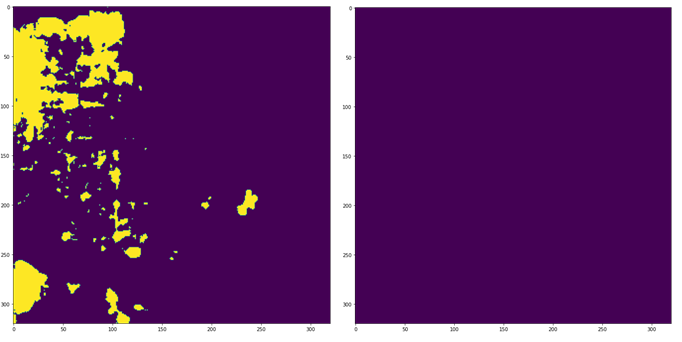
We finished training the model with an accuracy of 98.31% in the training dataset and 94.95% in the test dataset. Using the Jaccard or IoU index as a metric, we obtained 0.97 for the training dataset and 0.85 for the test dataset.


U-Net showed a good result in the segmentation of soyabean crop fields, even considering the presence of some false positives. To try to reduce these noises, we can collect more samples, which would make the model more robust. We can try to perform a preprocessing on the SAR image, using for example the Lee speckle filter. Another possible improvement is the use of other more complex architectures and with more parameters of neural networks for semantic segmentation, such as SegNet, HRNet, DeepLabV3+, ResUNet, etc.
Thank you!
LinkdIn Profile: https://www.linkedin.com/in/jo%C3%A3o-otavio-firigato-4876b3aa/
